The World Bank provides data on gross domestic product (GDP) per capita and life expectancy for various countries and regions of the world. An econometric analysis answers the question of how affluence relates to longevity.
The first section of this article presents results with brief economic interpretations, and the second section provides technical details on econometric methodology.
Executive Summary
The analysis finds that technological progress is a dominant factor of rising life expectancy. The effects of GDP growth emerge after removing this progress trend from the data. In industrial nations with highest GDP per capita, life expectancy drops by 8.3 days as a consequence of a 5% recession. Furthermore, it takes about 10 years until an economic contraction fully manifests. Developing nations with lowest GDP per capita are affected disproportionately harder. Here, life expectancy reduces by 69 days.
Results and Economic Interpretation
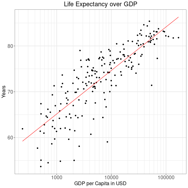
Updated for 2021, the World Bank publishes data on GDP per capita and life expectancy of 195 countries and territories. Plotting this data with GDP in a logarithmic scale reveals a clear relationship between higher GDP and longer lifetimes. In Figure 1 the red line indicates this trend.
On average, life expectancy rises by 2.41 months relative to a 5% increase in GDP per capita. Because of the dispersion of countries around the trend line, there is some uncertainty around this estimate. With 95% confidence, the true value falls in an interval between 2.19 and 2.64 months.
Note that at this point the statistic does not establish a causality between GDP and life expectancy. So average lifetimes do not rise by 2.41 months as a result of a 5% GDP growth. Similarly, we cannot conclude that countries are rich as a consequence of people living there growing older. We merely observe that, for whatever reasons, in countries with higher GDP per capita people tend to live longer.
Because the World Bank provides data starting in 1960, we can evaluate how the relationship has changed over time.
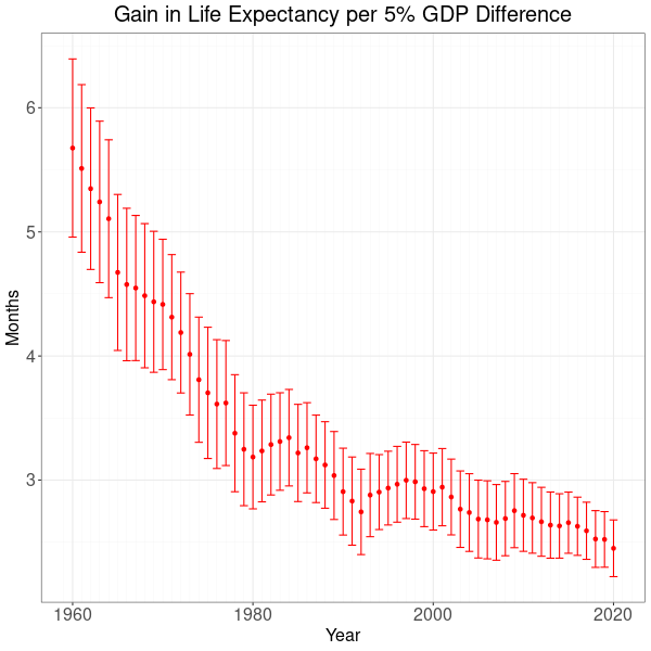
Figure 2 shows how the relationship between life expectancy and differences in gross domestic product has developed since 1960. While in 1960 life expectancy in countries with a 5% higher GDP rose by 5.7 months, by 2020 this difference had fallen to 2.4 months. Red dots mark best estimates and range bars denote 95% confidence intervals. This means that with a probability of 95% true values lie somewhere along the red lines for each of the years of the evaluation. Although confidence intervals reflect a degree of uncertainty, the general conclusion is that wealth promotes longevity.
However, the wealth effect has been trending downwards, which could be interpreted as a development towards more social justice. In 2020, differences between rich and poor impacted lifetimes to a lesser degree than in 1960. Interestingly, this positive trend reverses temporarily following recessions or periods of high interest rates in the US. Instances are the 1980 recession, the 1992 Sterling crisis, the burst of the .com bubble in 2000 as well as the 2008 financial crisis. Even the 2015 bounce might be attributed to the taper tantrum and subsequent instability in emerging markets. Economic downturns hit poorer countries harder because reduced incomes have a more direct impact on living conditions.
Social Policy Efficiency and Drivers of Longevity
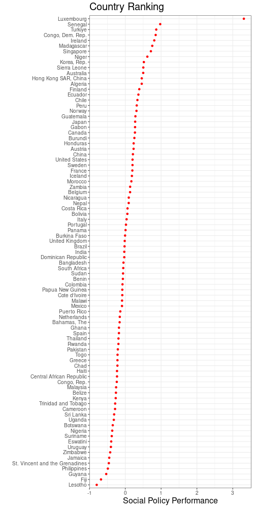
An interesting question is whether it is possible to derive a measure of social policy efficiency from the data. For if funding for social policy rises with GDP, then low GDP growth with high gains in longevity might be a measure for government policy aiming for social justice. However, a mapping of life expectancy growth to 2020 GDP per capita reveals another important general trend. Countries with low GDP per capita tend to have higher gains in longevity per GDP growth. The red trend line in figure 3 indicates how pronounced this difference between rich and poor countries is on average.
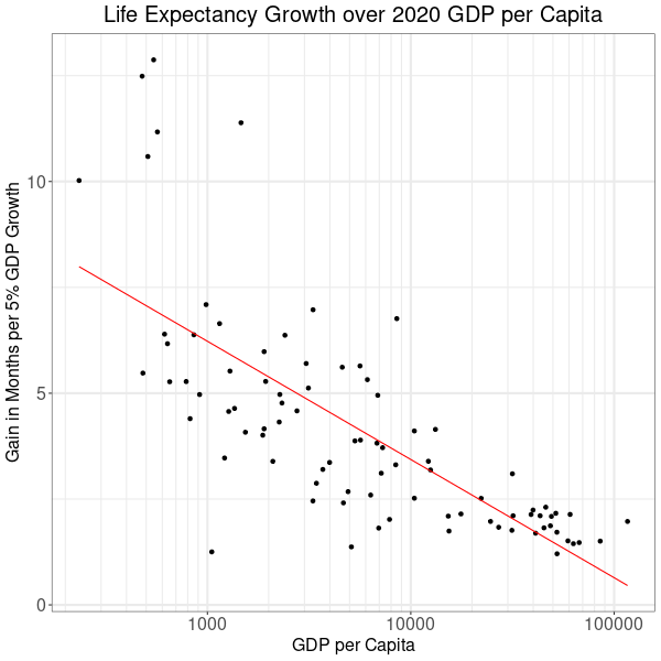
For a better understanding of the relationship, it helps to clarify what the axes in Figure 3 stand for. The vertical shows a ratio of the growths of life expectancy and GDP between 1960 and 2020. See the Technical Details section for mathematical definitions. In the following, the unit of the vertical axis is called life expectancy growth performance (LGP). Countries that had little gains in life expectancy but high GDP growth appear at the bottom end. Conversely, countries with low GDP growth but high gains in life expectancy end up at the top of the LGP scale. The GDP per capita generated by these countries in 2020 is plotted on the horizontal.
Countries that were rich in 2020 all cluster at the bottom right of Figure 3. Moving left, as countries become less affluent, their LGP rises along the trend line. Finally, the upper left has the group of top performers: the Democratic Republic of Congo, Madagascar, Senegal, Niger, Sierra Leone and Burundi.
The red trend line computed with a linear regression model says that on average, LGP sinks by 0.84 months when 2020 GDP per capita doubles. The 95% confidence interval for this value falls in between 0.67 and 1.01 months. So there is virtually no doubt that life expectancy grows less quickly as countries get richer.
Does this mean that GDP is bad for longevity? Of course not! When interpreting statistics, we must be mindful of causality. GDP is correlated to an omitted variable, which is the adoption of technical progress. The less developed a country, the more innovations that it can incorporate from the rest of the world. With regards to the outperforming African six, one might speculate that development aid could be an another important driver of life expectancy.
Summing up, technological progress is a main driver of rising life expectancy. Furthermore, the positioning of countries above or below the trend line in Figure 3 may yield some insight into how well countries conduct social policy programs. The technical details include a country ranking section derived from the LGP statistic.
Changing Life Expectancy as a Consequence of GDP Growth
This section examines how life expectancy changes as a consequence of GDP growth. Estimating this effect is complicated by the fact that technological progress is an important driver of life expectancy. Moreover, progress and economic growth are interdependent. Therefore, it is not possible to measure the influence of growth without taking account of progress.
Since progress is not observed in the data and hard to quantify, there is no option but to look for a proxy variable: time.
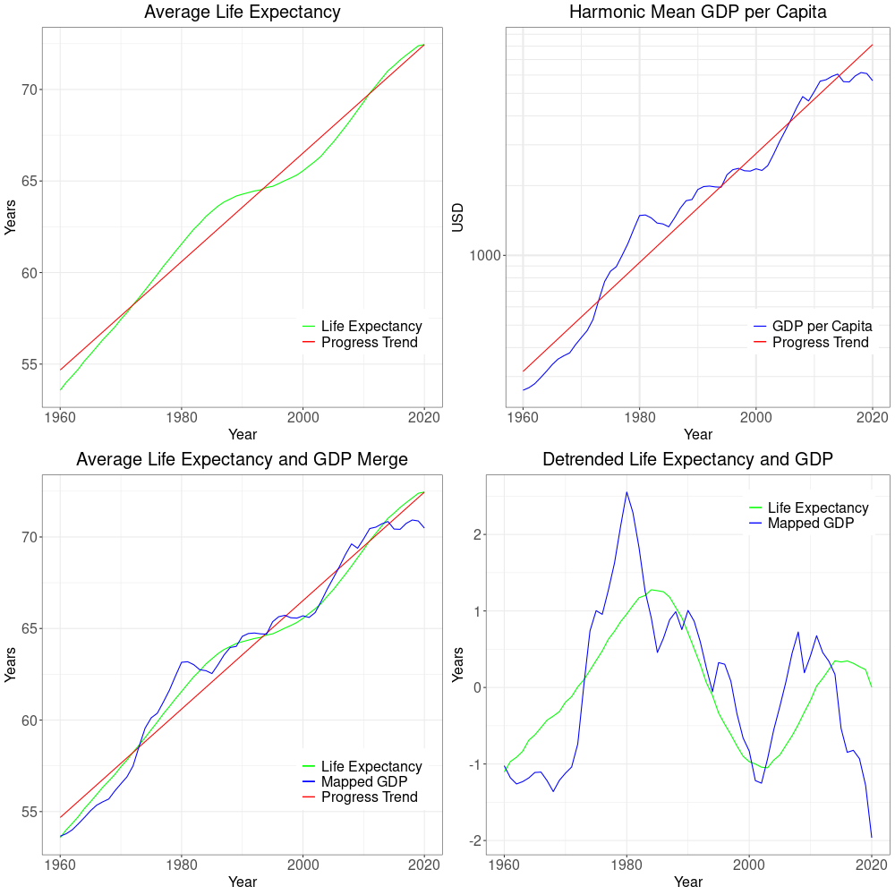
With time as a proxy, the first step to find the effects of GDP on longevity is to check how a linear progress trend relates to the overall changes. Figure 4 shows the workings of this method works applied to averages of 87 countries. The upper half has progress trends in red that best explain the rises in life expectancy and logarithmic GDP. Obviously, lifetimes and logarithmic GDP aren’t directly comparable. But mathematically it is straightforward to transform GDP data such that its trend line matches the one for life expectancy. In the lower left, Figure 4 shows the resulting mapping for GDP. Finally, in the lower right we see life expectancy and GDP with progress trends subtracted.
The progress trend indicates that between 1960 and 2020, on average life expectancy increased by 3.6 months per year for the 87 countries in scope.
Note how the removal of trends results in GDP and life expectancy averaging around zero. Furthermore, the curves in the lower right of Figure 4 do seem to correlate somewhat. That is, life expectancy rises and falls in a somewhat delayed manner with GDP.
In conclusion, trend removal is an essential step estimating the effects of fluctuations in GDP growth.
Effects of Economic Downturns on Life Expectancy
Estimating the impact of economic downturns necessitates trend removal. So the first step is to separate the effects of growth and progress by removing progress trends from the 87 countries with data between 1960 and 2020. Afterwards, a regression model measures to what extent deviations from trend GDP explain life expectancy.
Instead of working on country averages, trends will be removed for each of the 87 countries individually as this increases the sample size and yields superior results. And since life expectancy lags GDP, the statistical algorithm also checks after how many years the effects are most evident.
For the 87 countries as a whole, life expectancy drops by 31.1 days following a 5% GDP contraction, with 95% confidence of a true value between 18.4 and 43.9 days. Moreover, the effect appears to be strongest with a delay of one year. Note that the reduction of roughly one month due to a 5% drop in GDP is far below the 2.4 months that we arrived at previously. This is because the previous estimate included differences between countries in the adoption of progress.
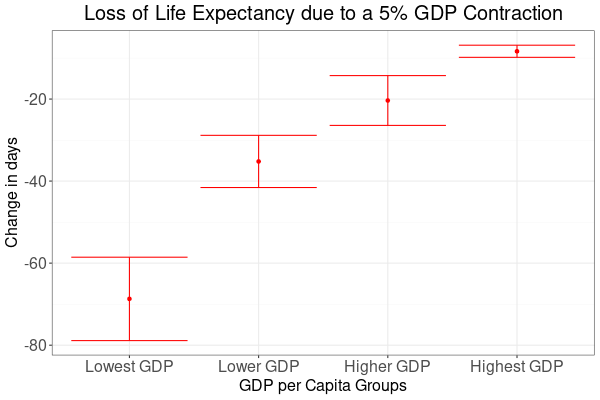
As observed in Figure 3, the growth of life expectancy depends on GDP per capita. It therefore makes sense to group countries by 2020 GDP per captia to see how differently economic crises affect richer and poorer nations.
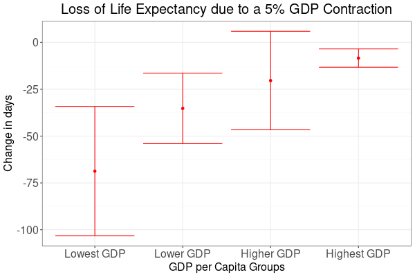
Figure 5 shows how crises affect lowest GDP countries disproportionately stronger. Again, the red dots indicate best estimates and the bars stand for confidence intervals. Unfortunately, due to distinctive heterogeneity estimates are not well defined, but still give an overall indication.
| Group | Estimate | 95% Confidence |
|---|---|---|
| Lowest GDP | 68.7 days | 34.2 to 103.3 days |
| Lower GDP | 35.2 days | 16.4 to 54.0 days |
| Higher GDP | 20.4 days | -5.94 to 46.7 days |
| Highest GDP | 8.35 days | 3.47 to 13.2 days |
To put these numbers into perspective, for a country like the US with a population of 330 million, an 8.3 day loss in life expectancy is equivalent to roughly 90,000 people dying a year earlier for each and every year that the effects of a 5% recession linger on. Or, if you wondered how 8.3 days could shorten life spans by a year, it would be 4.1 million dying early by those 8.3 days.
Speed of GDP affecting Life Expectancy
Further analysis allows to get a better idea of the speed at which economic crises manifest in changes to life expectancy. The previous analysis compared deviations from long term trends. Now, the investigation shifts to changes of these deviations by producing series of first differences from the detrended data. Using linear regression models on this data it is possible to explore how present and past changes in GDP relate to changes in life expectancy.
Results from an evaluation of first differences are much more robust than the previous assessment of overall deviations from long term trends. As can be seen in Figure 6, the upper limits of confidence intervals are all well below zero for the first 8 years. This means that it can be ruled out that results are mere coincidence without real world significance.
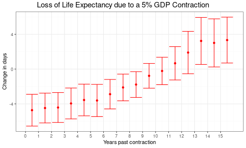
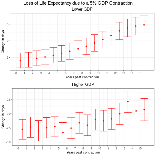
It takes roughly 10 years until a recession fully manifests in lost life expectancy for the 87 countries as a whole. Again, it makes sense to group countries by 2020 GDP per capita to see how the realization of economic shocks differs between richer and poorer countries.
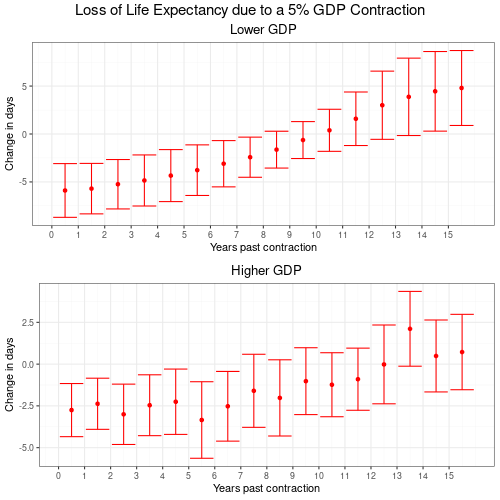
In Figure 7 comparing the speed of GDP shocks between lower and higher GDP per capita countries, the first thing to notice is the more regular realization of effects in lower GDP countries. Poorer countries are hit harder by recessions. But on the upside they appear to overcome the effects more rapidly and even offset some of the downside later on. In contrast, richer countries exhibit random variability and benefit to a lesser degree once they overcome a recession.
It might be an interesting field for further study if indeed lower GDP countries take less time to recover from recessions.
Technical Details
The regression of life expectancy on GDP per capita uses the following model:
LEi = β0   +  β1 * log(GDPi)  +  εi
     36.7    4.12
    (1.77)  (0.20)

LE: life expectancy in years
GDP: per capita GDP in current USD
i: country index

Coefficients for 2021
R2: 69%
The computations and regression model for life expectancy growth performance work as follows:
ΔGDPi = log(GDP2020i) - log(GDP1960i)
ΔLEi  = LE2020i - LE1960i
LGPi  = ΔLEi / ΔGDPi * log(1.05) * 12

LGPi  = β0    +   β1 * log(GDP2020i)  +  εi
      14.60     -1.213
     (1.066)    (0.1214)


ΔGDP: GDP change between 1960 and 2020
ΔLE:  Life expectancy change between 1960 and 2020
LGP:  Life expectancy growth performance
i:    Country index

R2: 54%
Country Ranking for Social Policy Performance
In Figure 3 the LGP of countries relative to the forecast trend line might be a somewhat useful measure for social policy performance. To get the performance measure, first subtract the forecast trend line from LGP data. Afterwards, divide the detrended data by the height of the trend. This yields, apart from Luxembourg, a relatively even distribution of performance measures. Figure 8 has the resulting ranking with country names. The outcome might reflect the combined effects of government policy and development aid to some degree.
Quantiles for Regressions with Progress Trends Removed
The four quantiles for regressions with progress trends removed have the following countries and territories:
Lowest GDP:
Benin, Burkina Faso, Burundi, Cameroon, Central African Republic, Chad, Democratic Republic of Congo, Haiti, Lesotho, Madagascar, Malawi, Nepal, Niger, Pakistan, Rwanda, Senegal, Sierra Leone, Sudan,
Togo, Uganda, Zambia, Zimbabwe.
Lower GDP:
Algeria, Bangladesh, Belize, Bolivia, Colombia, Republic of Congo, Cote d’Ivoire, Eswatini, Fiji, Ghana, Guatemala, Honduras, India, Jamaica, Kenya, Morocco, Nicaragua, Nigeria, Papua New Guinea, Philippines, Sri Lanka, Suriname.
Higher GDP:
Botswana, Brazil, Chile, China, Costa Rica, Dominican Republic, Ecuador, Gabon, Greece, Guyana, Malaysia, Mexico, Panama, Peru, Portugal, South Africa, St. Vincent and the Grenadines, Thailand, Trinidad and Tobago, Turkiye, Uruguay.
Highest GDP:
Australia, Austria, The Bahamas, Belgium, Canada, Finland, France, Hong Kong SAR China, Iceland, Ireland, Italy, Japan, Republic of Korea, Luxembourg, Netherlands, Norway, Puerto Rico, Singapore, Spain, Sweden, United Kingdom, United States.
Regression Models for Progress Trend Removal
To remove progress trends from life expectancy data, I used the following model:
LEit = βi0  +  βi1 * t + εit

LE: life expectancy
t: time in years
i: country index
The model to remove progress from GDP works in an analogous manner:
GDPit = βi0  +  βi1 * t + εit

GDP: log GDP per capita
t: time in years
i: country index
The regression models are then used to compute forecasts, which we subtract from the data to remove trends.
Regression Model for Effects of Economic Downturns on Life Expectancy
The regression model on the detrended data works with different lags on GDP to find the lag with the maximum impact:
LEit = β1 * GDPi(t-l) + εit

LE: life expectancy
GDP: log GDP per capita
i: country index
t: time index
l: lag between 0 and 15
For any group of m countries, an algorithm produces a series of data with lags between 0 and 15 years. Since the data has zero means we can use an OLS estimator for unbiased estimates of the coefficient β1. A simple technique for this is to append individual country series into one large set. This technique is computationally equivalent to a “within” estimator for panel data, see Verbeek (2004). One can then run estimates for all lags and select the biggest response. Alternatively, a panel estimator indexing on countries and years yields the same results.
However, this simplified OLS approach is not efficient for standard errors due to heterogeneity across groups. Given the differences between countries it should not come as a surprise that a Chow test rejects the null of constant slopes. Therefore, it is necessary to compute heteroskedasticity robust standard errors.
Since the detrended, but not yet differenced data exhibits very large differences between countries, standard errors not corrected for heteroskedasticity are way smaller. To see this, compare standard errors in Figure 5 to those in Figure 9.
Regression Model for Speed of GDP affecting Life Expectancy
The regression model for the speed at which GDP drops affect life expectancy is working on first differences.
ΔLEit = β1 * ΔGDPi(t-l) + εit

LE: life expectancy
GDP: log GDP per capita
i: country index
t: time index
l: lag between 0 and 15
Due to the differencing, estimates are less affected by heterogeneity. For this, compare Figure 7 to standard errors not corrected for heteroskedasticity in Figure 10.
References
A Guide to Modern Econometrics, Verbeek, 2nd Edition, 2004, Wiley
GDP per Capita: Worldbank.org
Life Expectancy at Birth: Worldbank.org